Un-0Unconventional AI's image generator. It integrates a field of coupled oscillators to a fixed point and reads the settled phases as pixels, rather than denoising or predicting tokens. generates images by integrating a field of coupled Kuramoto oscillatorsA population of phase oscillators that pull one another toward a shared rhythm through pairwise coupling. Un-0 integrates their dynamics and reads the settled phases as pixels. until phase synchronization occurs, then decoding the locked phases into pixels. The baseline CIFAR-10 model contains 19.4M parameters and takes 102 ms to generate a batch of 1,024 images on an NVIDIA A100 GPU.
Compressing Un-0 involves two complementary techniques: replacing the 16.8M parameter dense coupling matrix (86% of total model size) with a structured Monarch operator (0.52M parameters), and routing model matrix multiplications onto NVIDIA Tensor CoresDedicated matrix-multiply units on modern NVIDIA GPUs, several times faster than the general-purpose cores. A matmul must be dispatched to them explicitly. in mixed precision (BF16/TF32). Together, these changes shrink model size to 3.2M parameters (6.1× reduction) and reduce generation latency to 17.7 ms (5.77× speedup) while maintaining baseline clean-FIDA standardized FID implementation that fixes the resizing and preprocessing differences making raw FID incomparable across codebases. Lower is better. quality.
Phase synchronization during generation is visualized below. As the field settles, the order parameterThe Kuramoto synchronization measure r ∈ [0,1]: 0 when phases are scattered, 1 when they are perfectly locked. increases from 0 toward 1:
Evaluation Methodology & Quality Gates
All compression and optimization experiments were evaluated against Un-0’s clean-FID score on CIFAR-10. Maintaining quality parity was treated as a hard constraint: any optimization that degraded clean-FID was rejected, regardless of performance gains.
Analyzing Model Weight Distribution
Un-0 couples 4,096 phase oscillators using a learned dense coupling matrixThe learned matrix K whose entry Kᵢⱼ sets how strongly oscillator j pulls oscillator i. Here it is 86% of the model's parameters. of shape . This single matrix accounts for 16,777,216 parameters—86.3% of the model’s total 19,434,123 parameter budget. The remaining 2,656,907 parameters constitute the fixed backbone (natural frequencies and phase-to-pixel decoder):
| Config | Coupling K | Backbone (ω + decoder) | Total |
|---|---|---|---|
| Dense (released baseline) | 16,777,216 | 2,656,907 | 19,434,123 |
| Monarch depth-2 (shipped) | 524,288 | 2,656,907 | 3,181,195 |
| Monarch depth-3 + low-rank | 1,310,720 | 2,656,907 | 3,967,627 |
Backbone parameter count remains constant across all configurations at 2,656,907 parameters.
Applying is also the dominant runtime cost: generation performs 10 explicit Euler integration steps, applying twice per step (20 total applications of an operator per batch).
Why coupling is applied 20 times per generation step
Each generation step integrates the oscillator ODE over 10 explicit Euler steps. Evaluating the velocity equation requires applying the coupling matrix to two distinct activation vectors, sin(θ) and cos(θ), resulting in 2 coupling applications per integration step (20 applications total per batch).
Mathematical Derivation of Operator Structure
The Kuramoto velocity equation for oscillator is:
dθᵢ/dt = ωᵢ + Σⱼ Kᵢⱼ · sin(θⱼ - θᵢ)Applying the trigonometric angle-difference identity:
sin(θⱼ - θᵢ) = sin(θⱼ) · cos(θᵢ) - cos(θⱼ) · sin(θᵢ)Substituting this identity back into the velocity equation yields:
dθᵢ/dt = ωᵢ + cos(θᵢ) · (K · sin(θ))ᵢ - sin(θᵢ) · (K · cos(θ))ᵢThis expansion reveals that is consumed exclusively through linear operator products with activation vectors (K · sin(θ) and K · cos(θ)). Because individual matrix elements of are never accessed directly, can be replaced by any structured linear operator that supports fast matrix-vector products (K · v) with far fewer parameters, provided the operator is co-trained from scratch.
Mathematical derivation of the velocity expansion
Factoring out terms independent of index :
Σⱼ Kᵢⱼ · sin(θⱼ - θᵢ) = cos(θᵢ) · Σⱼ Kᵢⱼ · sin(θⱼ) - sin(θᵢ) · Σⱼ Kᵢⱼ · cos(θⱼ)
The resulting sums correspond directly to (K · sin(θ))ᵢ and (K · cos(θ))ᵢ. Diagonal elements K_ii contribute sin(0) = 0, making self-coupling dynamically irrelevant.
Monarch Factorization of the Coupling Matrix
Because is only evaluated as an operator, we can represent it using a Monarch factorizationWriting a dense matrix as a product of block-diagonal factors with a fixed permutation between them, so a matvec costs O(n^1.5) instead of O(n²).: a product of block-diagonalA matrix that is zero outside square blocks on its diagonal, so it mixes only within each block and applies as many small independent matmuls. matrices with fixed permutations. For , each factor consists of blocks of shape .
A depth-2 Monarch factorization requires two factors of 262,144 parameters each, reducing coupling parameter count from 16,777,216 down to 524,288 (a 32× parameter reduction for ):
- Coupling matrix (): 16,777,216 → 524,288 parameters (32.0× reduction).
- Total model: 19,434,123 → 3,181,195 parameters (6.11× reduction).
- Coupling K (16.78M)86.3%
- Backbone: ω + decoder (2.66M)13.7%
- Coupling K (0.52M)16.5%
- Backbone: ω + decoder (2.66M)83.5%
Monarch factorization mechanics and low-rank residuals
A depth-2 Monarch factorization decomposes an matrix into , where and are block-diagonal and is a transpose permutation matrix. Computing requires operations instead of .
To allow mixing across block boundaries, we include an optional low-rank residual initialized with (LoRA-style). Co-training the structured operator from scratch allows the network to adapt its weights to this factorization.
Memory-Bound vs Launch-Bound Performance Characteristics
Parameter reduction alone does not produce proportional wall-clock speedups. In FP32 execution without Tensor Core dispatch, the Monarch model reduces A100 batch-1024 generation latency from 102.2 ms to 64.9 ms (a 1.57× speedup despite a 6.1× parameter drop).
Monarch factorizations decompose matrix multiplication into many small block matmuls. At small block sizes, execution becomes launch-boundA regime where wall-clock is set by the fixed cost of launching each GPU kernel, not by the arithmetic inside it., where kernel launch and scheduling overheads dominate computation time. Furthermore, small block operations default to memory-bound GEMVGEMV is a matrix-vector product: memory-bound and small. GEMM is a matrix-matrix product: compute-bound, and maps onto the tensor cores. Monarch's small blocks lower to a GEMV by default, leaving the fast units idle. routines on standard CUDA cores rather than Tensor Core GEMM kernels.
Kernel launch overheads in small-block factorizations
While dense matrix multiplications execute as a single saturated GPU kernel, depth-2 Monarch factorizations execute dozens of small block launches. Below threshold matrix sizes, kernel invocation overheads dominate GPU execution time. Converting parameter reduction into wall-clock speedup requires dispatching block operations to Tensor Cores.
Tensor Core Dispatch & Mixed Precision Execution
The baseline Un-0 implementation runs FP32 computations on general CUDA cores, leaving GPU Tensor Cores unused. Enabling TF32TensorFloat-32, a reduced-precision matmul mode that runs on the tensor cores while keeping fp32's range. Switching it on lets matmuls dispatch to the fast units. precision and BF16bfloat16, a 16-bit floating-point format that runs on the tensor cores. Here it is the deploy precision, gated on FID. autocast routes matrix multiplications to cuBLAS Tensor Core kernels, while torch.compile fuses surrounding element-wise trigonometric operations.
Deploying the depth-2 Monarch model with Tensor Core dispatch cuts generation time on an A100 (1024-batch) from 102.2 ms to 17.7 ms (5.77× speedup relative to baseline):
Interaction between Tensor Core dispatch and library kernels
Switching execution to BF16/TF32 allows PyTorch to select hardware-accelerated cuBLAS routines. torch.compile fuses element-wise sin, cos, and scaling operations around these calls, eliminating intermediate memory round-trips.
Empirical Quality Parity & Checkpoint Selection
Model quality was evaluated using clean-FID across 50,000 class-balanced CIFAR-10 samples across multiple random seeds. The baseline dense checkpoint scores 8.88 (FP32 min).
The depth-2 Monarch model achieves a clean-FID score of 8.93 (FP32 min), remaining within the ~0.1 seed variance margin of the baseline:
Evaluation of Higher-Depth Monarch Configurations
We also evaluated a depth-3 Monarch configuration with an added rank-64 residual (1,310,720 coupling parameters, 3.97M total parameters). At its best converged checkpoint (epoch 1200), depth-3 achieved clean-FID scores of 9.00 / 9.04 (min / mean), performing slightly worse than the depth-2 model (8.93 / 8.99). Because depth-3 added parameter overhead without improving quality, the depth-2 configuration was selected for deployment.
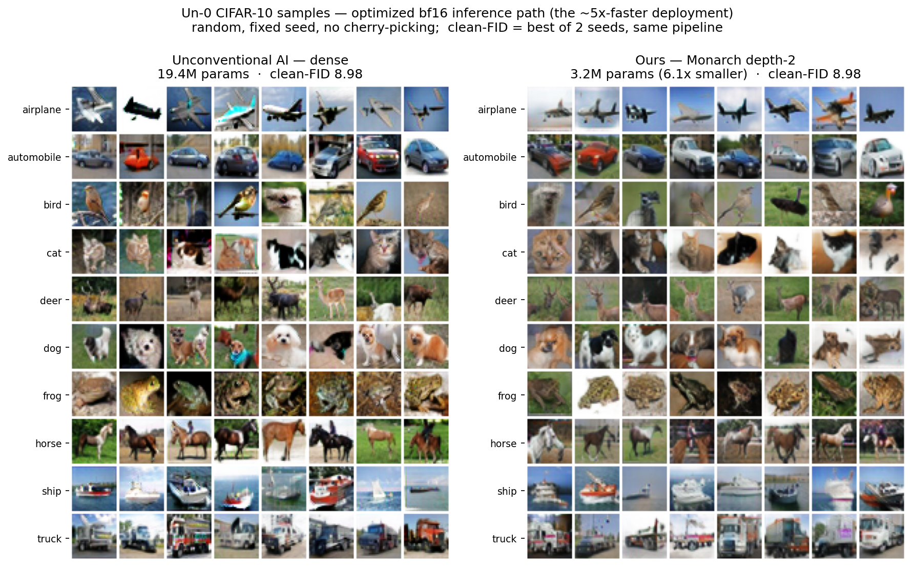
On the target BF16 deployment path, both dense baseline and depth-2 Monarch models achieve matched clean-FID scores of 8.98:
| Model | Params | FID (FP32) | FID (BF16 deploy) | BF16 Delta |
|---|---|---|---|---|
| Dense baseline | 19.43M | 8.88 | 8.98 | +0.09 |
| Monarch depth-2 (shipped) | 3.18M | 8.93 | 8.98 | +0.05 |
| Monarch depth-3 + low-rank | 3.97M | 9.00 | N/A | N/A |
Clean-FID scores are matched at 8.98 on the BF16 deployment path.
Throughput benchmarking on NVIDIA A100 and T4 GPUs confirms speedups across hardware platforms:
Custom GPU Kernel Profile & Amdahl Analysis
Profiling execution under torch.compile on an A100 (18.41 ms total per batch) reveals that GPU compute accounts for 11.86 ms (64.4%), while host-side Python iteration overhead accounts for 6.55 ms (35.6%):
- GPU active compute64.4% · 11.86 ms
- Host CPU idle overhead35.6% · 6.55 ms
Within active GPU execution time, coupling matrix evaluation remains the single largest component (23.2% of GPU time).
We evaluated custom Triton kernels to fuse depth-2 Monarch operations into fewer launches. In isolation, a custom Triton kernel executed the coupling step 1.34× faster than torch.compile.
However, applying Amdahl’s LawThe cap on end-to-end speedup from optimizing only part of a workload. A 1.34× kernel on a 23% slice yields at most about 1.1× overall. to a 23.2% compute slice caps theoretical end-to-end speedup at ~1.06× (~1.1×). Furthermore, custom kernels do not reduce host CPU launch overhead.
Amdahl's Law calculation for coupling kernel speedup
Given coupling execution fraction of GPU active time and kernel speedup :
End-to-end speedup = 1 / ((1 - p) + p/s) = 1 / (0.768 + 0.232 / 1.34) = 1.063×
Even an instantaneous coupling kernel () would yield a maximum overall speedup of on active GPU time.
When extending custom kernels to cover surrounding element-wise operations (sin, cos, scaling), torch.compile (via PyTorch Inductor) outperformed hand-written kernels by reusing intermediate trigonometric values and optimizing tile sizes. Consequently, custom coupling kernels were not included in production builds.
Solver Loop Bottlenecks & Future Optimization
Because host-side loop overhead and step counts dominate remaining runtime, future speedups rely on ODE solver step reduction.
Un-0 currently executes 10 explicit Euler integration steps. Reducing integration from 10 steps to 7 or 6 steps offers projected speedups of 1.43× and 1.67× respectively:
Step reduction requires re-validating clean-FID scores to ensure output quality remains within acceptable bounds.
Summary of Compression Results
| Configuration | NVIDIA A100 (batch 1024) | NVIDIA T4 (batch 1024) |
|---|---|---|
| Tensor Core dispatch (no model changes) | 4.82× speedup (21.2 ms) | 3.36× speedup |
| Monarch compression only (FP32) | 1.58× speedup (64.9 ms) | N/A |
| Full stack (Monarch + Tensor Cores) | 5.77× speedup (17.7 ms) | 4.97× speedup |
| Parameter count reduction | 6.11× smaller (19.4M → 3.2M) | Same |
| Clean-FID quality (BF16 deploy) | 8.98 (matched baseline) | Same |
Full stack achieves 17.7 ms batch latency on A100 and 6.1× parameter reduction at matched clean-FID (8.98).
Glossary
Glossary — every term, defined
- Un-0
- Unconventional AI's image generator. It integrates a field of coupled oscillators to a fixed point and decodes the settled phases into pixels, rather than denoising (diffusion) or predicting tokens (autoregression).
- Kuramoto oscillators
- A population of phase oscillators, each with a phase θ and a natural frequency ω, that pull one another toward a shared rhythm through pairwise coupling.
- Coupling matrix (K)
- The learned matrix whose entry
Kᵢⱼsets how strongly oscillator j pulls oscillator i. At n=4096 it is 16.8M parameters, 86% of the model. - Order parameter (r)
- The Kuramoto synchronization measure r ∈ [0,1]: 0 when phases are scattered, 1 when they are perfectly locked. The live canvas shows it climbing as the field settles.
- Angle-difference identity
sin(θⱼ−θᵢ) = sinθⱼ·cosθᵢ − cosθⱼ·sinθᵢ. Expanding the coupling this way shows K is only ever used asK·sinθandK·cosθ, never as a materialized matrix.- Monarch factorization
- Writing a dense matrix as a product of block-diagonal factors with a fixed permutation between them, so a matvec costs O(n^1.5) instead of O(n²). Here the coupling is a depth-2 Monarch product.
- Block-diagonal
- A matrix that is zero outside square blocks on its diagonal, so it mixes only within each block and applies as many small independent matmuls.
- Low-rank residual
- An optional global channel
(x·V)·Uᵀadded to the Monarch product, with U zero-initialized so the operator starts as pure Monarch and grows the global path only if training asks. - FID
- Fréchet Inception Distance, the standard image-generation quality metric. Lower is better.
- clean-FID
- A standardized FID implementation that fixes the resizing and preprocessing differences that make raw FID scores incomparable across codebases. The metric Un-0 is judged on.
- bf16 / TF32
- Reduced-precision floating-point formats that run on the tensor cores. bf16 is the deploy precision, gated on FID at a measured tax of ≤0.1. This is inference precision only, not weight quantization.
- Tensor cores
- Dedicated matrix-multiply units on modern NVIDIA GPUs, several times faster than the general-purpose cores. A matmul must be dispatched to them explicitly.
- GEMV vs GEMM
- GEMV is a matrix-vector product: memory-bound and small. GEMM is a matrix-matrix product: compute-bound and maps onto the tensor cores. Monarch's small blocks lower to a GEMV by default.
- Launch-bound
- A regime where wall-clock is set by the fixed cost of launching each GPU kernel, not by the arithmetic inside it. Monarch's many tiny block matmuls are launch-bound.
- Amdahl ceiling
- The cap on end-to-end speedup from optimizing only part of a workload. A 1.34× kernel on a 23% slice yields at most ~1.1× overall.